Introduction

On one of my favorite wargame websites has a series of challanges on breaking CAPTCHA. It starts with a straightforward challange:

Please enter the CAPTCHA backwards

Time remaining: 10.00 seconds

Since no distortions are introduced to the text and there are ~100 distinct shapes, there are plenty of ways to read the text off the image without resorting to machine learning.

The next one is even easier - only 12 distinct shapes:

Please enter the CAPTCHA using the key provided

Time remaining: 10.00 seconds

Key: 😃 :D | 🙂 :) | 😋 :p | 🙁 :( | 😉 ;) | 😎 B) | 😡 :@ | 😮 :o | 😖 :s | 😐 :| | 😕 :/ | 💚 <3

Then there are a couple of other similar challanges, each one slightly harder than the previous. Until, finally, there is this challange:

Please enter the CAPTCHA using the key provided

Time remaining: 10.00 seconds

Key: 😃 :D | 🙂 :) | 😋 :p | 🙁 :( | 😉 ;) | 😎 B) | 😡 :@ | 😮 :o | 😖 :s | 😐 :| | 😕 :/ | 💚 <3

I couldn’t think of any bruteforce solution to this. Different symbol colors, translations and rotations makes a number of distinct shapes that can appear on an image very large. Here, a distinct shape means a unique ordering of pixel values in the image including their orientation.

At the same time, this seems to be a perfectly manageable task for a convolutional neural network (CNN or ConvNet). A CNN can learn a representation of an image that is invariant to small transformations, distortions and translations in the input image.

SPOILER ALERT: I really enjoyed solving this challenge and don’t want to spoil it for others. If you want to try solving this challenge, here is the website that hosts it. It’s in CAPTCHA category there.

If you are not very interested in attempting the challange, but want to see a simple application of a CNN that is different from MNIST or CIFAR-10 classification (I have read way too many tutorials on these), then continue reading!

Imports

This post was written in 2017. Keras changed quite a lot since then. Just a FYI.

import numpy as np
import glob
from scipy import misc
import matplotlib.pyplot as plt 
import os
from random import randint
from keras import utils
from keras.preprocessing.image import ImageDataGenerator
from keras.models import Sequential, load_model
from keras.layers import GlobalAveragePooling2D, Activation, Conv2D, MaxPooling2D
from keras.losses import categorical_crossentropy
from keras import losses
from keras import callbacks
from keras import optimizers
from imageio import imread

Getting the Training Data

What I like a lot about this series of challanges is that there is no additional data provided. The only piece of data at my disposal is a single 450x60px CAPTCHA image that changes as the webpage is refreshed. This is a very unusual situation for a person who is used to applying machine learning in situations when lots of training data is available (e.g. assignments for online courses, Kaggle challanges).

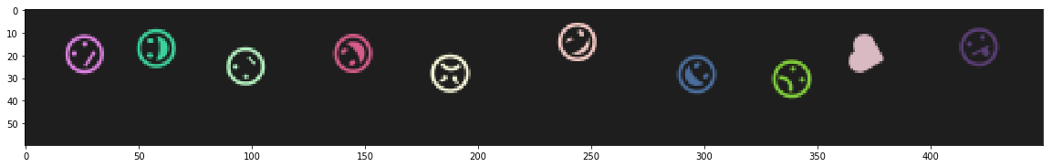
No programming was involved for this part. Since there are 12 different symbols and an immense number of ways how they can appear on the image, the best I can do at this point is to get a single example of each symbol. I download several images and use GIMP to cut out 20x60px parts, each containing a single symbol. The choice of cut out image dimensions is not arbitrary; it is required to make the object detection algorithm that I use later to work. As mentioned earlier, the height of a CAPTCHA image is 60px; each symbol has a diameter of 17-18px. So a resulting 20x60px image, that is centered horizontally on a symbol, has this symbol fully inside the image with an arbitrary vertical translation. Then I used GIMP to center the symbol vertically. I am pretty sure that the last step is not required, but it simplifies the process of augmented data generation and (probably) speeds up the training process as a result.

Here is the result of manual training data collection and initial preprocessing:

Training Data Preprocessing

This was the most challanging part of the challange for me. Since I didn’t have the resources to collect and label a dataset large enough to train an unbiased model, I decided to generate training data that would look like it came from the same distribution as original symbols in the CAPTHCA image.

Tensor image data generator that is provided by Keras library is good at adding translational and rotational augmentations to generated data. The next section describes that process in detail. However, this image data generator doesn’t have built-in capabilities that allow color augmentation. And I couldn’t think of a preprocessing function that would generate color that comes from the same distribution as color in CAPTCHAs. The easiest solution left is to eliminate color altogether with the help of the following functions:

# RGB to grayscale conversion
def rgb2gray(rgb):
    return np.dot(rgb[...,:3], [0.299, 0.587, 0.114])

def img_preprocess(img):
    img_no_alpha = img[:,:,0:3] # Strip 4-th channel (alpha). Shape is (60,20,3)
    img_gray = rgb2gray(img_no_alpha) # Outputs matrix of shape (60,20)
    img_gray[img_gray <= 30] = 0 # Make background black
    img_gray[img_gray > 30] = 255 # Make the rest white
    img_processed = img_gray / 255 # Center pixel values
    return img_processed

It’s possible to import a rgb2gray() function from an existing library, i.e. color.rgb2gray in scikit-image library. That implementation centers the image tensors (the output pixel values become floats in a range [0,1]). I preferred to center the image tensors as a last step in preprocessing, so I defined my own function.

Now on to loading 12 training images and some further preprocessing.

%matplotlib inline

train_data_path = '/data/train/*'
abs_path = os.getcwd()
path = abs_path + train_data_path

img_arr = []

for img_file in glob.glob(path):
        train_img = imread(img_file) # Outputs tensor of shape (60,20,4)
        train_img_processed = img_preprocess(train_img)
        img_arr.append(train_img_processed)

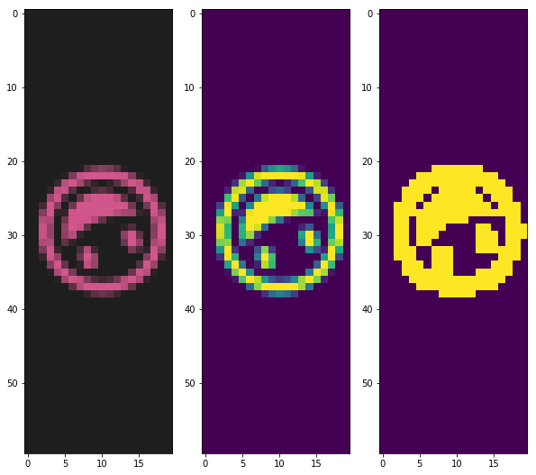
Here are images of intermediate results to help understand the preprocessing steps.

# Show original RGB image
plt.figure(1, figsize=(10, 10))
plt.subplot(131)
plt.imshow(train_img)

# Show grayscale image. Some limited information about original color is still preserved.
plt.subplot(132)
plt.imshow(rgb2gray(train_img))

# Show final processed image that has only two possible pixel values - 0 or 1.
# No color information is preserved while the general shape of the symbol is.
plt.subplot(133)
plt.imshow(train_img_processed)
plt.show()

There are a few more steps left to make this training data work with Keras.

def img_arr_to_4D(img_arr):
    X = np.stack(img_arr, axis=2) # Stack along 3-rd dimension. Outputs tensor of shape (60,20,12)
    X = np.rollaxis(X, 2) # Changes tensor shape to (12,60,20). Keras with Tensorflow backend needs this format.
    X = np.expand_dims(X, 3) # Add a fourth dimension. Conv2D() accepts 4D tensors only as input.
    return X

X_train = img_arr_to_4D(img_arr)
X_train.shape

(12, 60, 20, 1)

Now that the training data is preprocessed and in Keras-friendly format, it needs to be labeled. The labels and their order may seem a bit weird. There are lots of different ways to label this data. I chose a simple mapping: 0 ⇒ :D, 1 ⇒ :) and so on. Numbers in my mapping correspond to the order in which the symbol to string mapping is shown in the challange.

Y_train = np.array([0,1,10,11,2,3,4,5,6,7,8,9]) # Label training examples
Y_train = utils.to_categorical(Y_train, num_classes=12) # Converts a class vector to one-hot matrix

As for the order of labels in the Y_train array, it is the way it is because of the order in which the images were loaded in the for-loop in code section 19. First 0.png was loaded, then 1.png, 10.png, 11.png, 2.png and so on.

Augmented Data Generation

Training neural networks requires large amount of training data; certainly larger than 12 examples that were extracted manually.

The problem of varying color was solved at preprocessing step by applying a grascale filter and then limiting the pixel values to only two possible states (0 or 1). Now, the training data needs to represent all 12 possible symbols with two types of image transformations applied: random shifts along the vertical axis and random rotations.

It is possible use ImageDataGenerator to generate batches of augmented tensor image data at training time.

Here is how I defined the generator:

datagen = ImageDataGenerator(height_shift_range=0.50, width_shift_range=0.02, 
                                 rotation_range=360, fill_mode='constant', cval = 0)

The arguments are easy to understand:

• height_shift_range=0.50 - image data can be shifted randomly along the vertical axis by 50% of its total height at most.

• width_shift_range=0.02 - image data can be shifted randomly along the horizontal axis by 2% of its total width at most. This argument is not strictly required. Because of the way the sliding window reads the test data, a symbol will always be centered horizontally in the 60x20 image. I added this as a countermeasure for possible overfitting.

• rotation_range=360 - image data can be rotated randomly by 360° at most. I am not sure if random rotations happen in both directions (in such case 180° would suffice).

• fill_mode='constant - when an image is rotated or shifted, there will be data points outside of boundaries of an input. They are going to be filled with zeroes (background color)

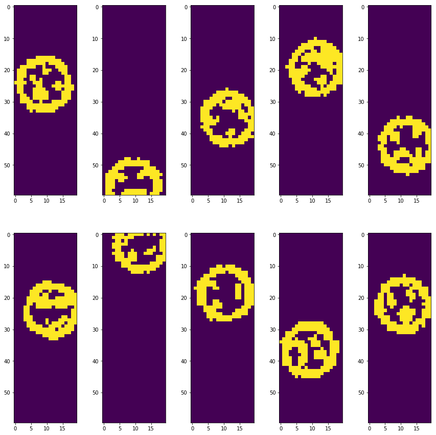
• ImageDataGenerator generates augmented image data in real time during training and can do so indefinitely. It is useful to have a rough idea of what kind of augmented data will be supplied to the CNN. ImageDataGenerator’s flow() method returns NumpyArrayIterator which can be used to generate and view a sample of augmented image data.

datagen_iter = datagen.flow(X_train, batch_size=10)

datagen_sample = datagen_iter.next()

plt.figure(1, figsize=(15, 15))

for i, img in enumerate(datagen_sample):
    plt.subplot(2,5,i+1)
    plt.imshow(img[:,:,0])

CNN Model Architecture

I started studying CNNs only a few weeks before I attempted this challange. Naturally, I didn’t have a good intuition about what constitutes a good CNN model architecture, apart from simple facts that apply to all neural networks: use bigger network to avoid bias, use more data to avoid overfitting.

I decided to simply copy a model I like from some whitepaper. According to Andrej Karpathy, this is a very solid approach for practical applications. Since my problem is relatively simple, I don’t need to use a model that performs well on some complex dataset, like ILSVRC. I searched for a model that does reasonably well on CIFAR-10 since it is a popular dataset that is somewhat similar to mine. CIFAR-10 consists of 60000 32x32 colour images in 10 classes. My dataset consists of an arbitrarily large number of 60x20 grayscale images in 12 classes.

I skimmed through a couple of papers until I stumbled on the one I really liked: Striving for Simplicity: The All Convolutional Net. The authors were looking to simplify conventional approach to model architecture. They decided not to use fully-connected layers at the higher layers of the network in order to reduce the number of parameters in the network. It suited me well, since I didn’t want to spend lots of time training the network on my laptop. I tried several models from that paper (model descriptions appear on pages 3 and 4), including All-CNN model which uses convolutional layers only (for downsampling it uses convolutional layers with stride larger than 1). In the end, I went with the base model C (page 3). It offered fastest initial learning rate and has only ~950,000 parameters, which is very impressive.

model = Sequential()
model.add(Conv2D(96, kernel_size=(3, 3), activation='relu',
                padding = 'same', input_shape=(60,20,1)))
model.add(Conv2D(96, (3, 3), activation='relu', padding = 'same'))
model.add(MaxPooling2D(pool_size=(3, 3), strides = 2))
model.add(Conv2D(192, (3, 3), activation='relu', padding = 'same'))
model.add(Conv2D(192, (3, 3), activation='relu', padding = 'same'))
model.add(MaxPooling2D(pool_size=(3, 3), strides = 2))
model.add(Conv2D(192, (3, 3), activation='relu', padding = 'same'))
model.add(Conv2D(192, (1, 1), activation='relu'))
model.add(Conv2D(12, (1, 1), activation='relu'))
model.add(GlobalAveragePooling2D('channels_last'))
model.add(Activation(activation='softmax'))

# Model architecture summary:

model.summary()

_________________________________________________________________
Layer (type)                 Output Shape              Param #   
=================================================================
conv2d_8 (Conv2D)            (None, 60, 20, 96)        960       
_________________________________________________________________
conv2d_9 (Conv2D)            (None, 60, 20, 96)        83040     
_________________________________________________________________
max_pooling2d_3 (MaxPooling2 (None, 29, 9, 96)         0         
_________________________________________________________________
conv2d_10 (Conv2D)           (None, 29, 9, 192)        166080    
_________________________________________________________________
conv2d_11 (Conv2D)           (None, 29, 9, 192)        331968    
_________________________________________________________________
max_pooling2d_4 (MaxPooling2 (None, 14, 4, 192)        0         
_________________________________________________________________
conv2d_12 (Conv2D)           (None, 14, 4, 192)        331968    
_________________________________________________________________
conv2d_13 (Conv2D)           (None, 14, 4, 192)        37056     
_________________________________________________________________
conv2d_14 (Conv2D)           (None, 14, 4, 12)         2316      
_________________________________________________________________
global_average_pooling2d_2 ( (None, 12)                0         
_________________________________________________________________
activation_2 (Activation)    (None, 12)                0         
=================================================================
Total params: 953,388
Trainable params: 953,388
Non-trainable params: 0
_________________________________________________________________

The model uses categorical crossentropy loss function, since the problem is a discrete classification task in which the classes are mutually exclusive. Adam optimizer is used, since it is very popular among the researchers and I have a good understanding of how it works. Accuracy is used to measure the model’s performance during training, so we know when to stop (the training can go on forever since the training data is generated in real time).

model.compile(loss=losses.categorical_crossentropy,
                  optimizer=optimizers.Adam(),
                  metrics=['accuracy'])  

The following code creates a callback function that saves the model during training. I decided to save every 5th model and only if it’s better than the previous saved one. Each model is ~80M so the size of the checkpoints directory can grow really quickly if the training rate is slow.

filepath = 'models/captcha4.{epoch:02d}-{loss:.2f}.hdf5'
checkpoint = callbacks.ModelCheckpoint(filepath, monitor='loss', verbose=0, 
                                                 save_best_only=True, mode='auto', period=5)

CNN Model Training

Finally, everything is set up for training!

The next function trains the model using the data generated by datagen image generator that was defined earlier. The choice of the batch size and the number of steps per epoch is mostly arbitrary. Usually it is advised to have a bigger batch size, if you can afford it, since the gradient descent will move more smoothly towards the local optima. I set the batch size to be pretty low since I tried out lots of different models and wanted to see quickly if they work well or not.

The number of epochs does not really matter as checkpoints are created along the way and the training can be stopped at any time.

80% accuracy can be obtained after only 30 or so epochs. After 30 minutes of training (100 epochs) the gradient descent slows down; the model has a training accuracy of ~95% at that point. Around epoch 150 it seems like the gradient descent converges to a model with ~98-99% training accuracy, >0.05 training loss. I ran the model for 500 epochs in total and did not see any substantial improvement. The model that is loaded in the last section of this notebook has an accuracy of >99% and <0.01 loss (saved at epoch 250).

# Only run if you are ready to wait for at least 30 minutes

#model.fit_generator(datagen.flow(X_train, Y_train, batch_size=15),
#                    steps_per_epoch=60, epochs=10000, callbacks = [checkpoint], use_multiprocessing=True)

Here are Tensorboard visualisations of the training process. Y-axis is loss/accuracy, X-axis is # of epochs.

Model Testing: Individual Symbol Detection

The CAPTCHA challange has a clearly defined objective: the correct CAPTCHA has to be submitted to the website during a 10-second time period after the webpage is reloaded. Therefore, no test set was created, nor did I measured the test performace using any conventional metric. I wrote a function (not included in this write-up) that authenticates on the website, reloads the webpage with CAPTCHA, gets CAPTCHA image and passess it to another function along with the trained model. That function uses the model to read the CAPTCHA, outputs its contents as a string which is then posted to the webpage. My only “performance metric” was a string at the top of the webpage which indicated whether the challange is “Incomplete” or “Complete”.

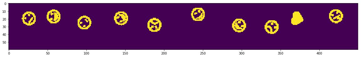
First, test image needs to be loaded. Instead of getting a new image directly from the website, like I did for the actual challange, 1 of 5 images that I downloaded in advance is randomly selected and used for testing in this notebook.

test_img_file = 'data/examples/captcha4_{}.png'.format(randint(1, 5))
test_captcha = imread(test_img_file) # Load (60, 450, 3) image
test_img = img_preprocess(test_captcha) # Apply same preprocessing as to train images. Output is (60, 450)

plt.figure(1, figsize=(20, 20))
plt.imshow(test_img)

The following code represents a very rudimentary approach to individual symbol detection in the 450x60 RGB CAPTCHA image that is presented on the challange’s webpage. I didn’t have a chance to research more advanced methods for object detection, so I came up with my simple implementation of sliding window. I don’t like that it requires very specific conditions to be fulfilled; the train image size and some image preprocessing steps were there just to make this method work. But it works for this particular task, which is what really matters in the end.

First, some variables that are used by the sliding window are defined. The most important variable is dark strip. It is a column vector of length 60 filled with zeros. It is going to be used to check if edges of the moving window and the moving window’s center intersect any symbol.

dark_strip = np.zeros((60, 1), dtype='float64')  # Create black vertical strip of dim 60x1 
window_width = 20 # Sliding window width
img_width = test_img.shape[1] # 450 pixels
img_arr = []

The width of the sliding window is 20 pixels and symbols are usually 17-18 pixels wide, therefore we can be certain that a symbol is within the window’s edges completely when the window’s edges don’t intersect anything, but a vertical strip at the window’s center intersects something. The following visualisation can be helpful to understand how it works:

The window moves from left to right one pixel at a time. When it detects a symbol, it saves the contents of the window to an array and jumps over 20 pixel (since that horizontal stretch is already saved). In the visualisation, the window’s edges are represented by two red lines, the window’s middle is represented by a red line that is yellow in parts where it intersects a symbol. In this particular example the window has detected a symbol: both edges are not intersecting anything but the center line intersects the symbol.

# Sliding window
window_left_edge = 0 # Starting position is at leftmost end of the image

while window_left_edge < (img_width - window_width):

    window_right_edge = window_left_edge + window_width # Make window 20 pixels wide at its current position
    window_middle = window_left_edge + (window_width // 2)

    left_clear = np.all(test_img[:,window_left_edge] == dark_strip) # Check if window's left edge is clear
    right_clear = np.all(test_img[:,window_right_edge] == dark_strip) # Check if window's right edge is clear
    center_not_clear = np.any(test_img[:,window_middle] != dark_strip) # Check if window's center intersects something
    
    # Check that left and right strips are dark and center strip is not dark (means centered on symbol)
    if (left_clear and right_clear and center_not_clear):
        img_arr.append(test_img[:,window_left_edge:window_right_edge]) # append the contents of the window to array
        window_left_edge = window_right_edge # can jump over the next 20 pixels as window detected symbol here
        
    window_left_edge += 1 # Move window by 1 pixel to the left   

# Stack captured test images into a single numpy array
X_test = img_arr_to_4D(img_arr)
X_test.shape # Check that 10 symbols were captured

(10, 60, 20, 1)

# Show what sliding window captured
plt.figure(1, figsize=(15, 15))

for i, img in enumerate(X_test):
    plt.subplot(2,5,i+1)
    plt.imshow(X_test[i,:,:,0])

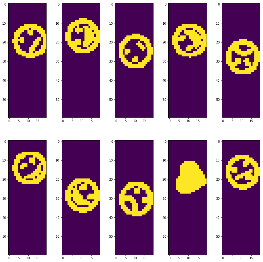
Looks like the sliding window captured every symbol from CAPTCHA image; and these images have dimensions 20x60, the same that were used in training! Here’s the entire processed CAPTCHA image again to make sure that nothing is missing.

plt.figure(1, figsize=(20, 20))
plt.imshow(test_img)

Model Testing: Prediction

All the hard work is done at this point. The only thing left is to load a pre-trained model and apply it to data extracted in the previous section.

model = load_model('models/captcha4.249-0.00.hdf5') # Load pre-trained model (loss: <0.01 after 165 epochs)
pred = model.predict(X_test, batch_size = 12) # Predict label probabilities for each image 
pred = np.argmax(pred, axis=1) # Select label with highest probability

# Define mapping that was introduced back in Training Data Preprocessing section.
mapping = {0: ':D',
           1: ':)',
           2: ':p',
           3: ':(',
           4: ';)',
           5: 'B)',
           6: ':@',
           7: ':o',
           8: ':s',
           9: ':|',
           10: ':/',
           11: '<3'
        }

# Print answer to CAPTCHA
answer = ''

for label in pred:
    answer+=mapping[label]
    answer+=' ' # Add spaces for easier comprehension
print('CAPTCHA: {}'.format(answer))

# Print CAPTCHA image for visual evaluation
plt.figure(1, figsize=(20, 20))
plt.imshow(test_captcha)

CAPTCHA: :/ :D :| :D :@ :D :D :( <3 :p 

You can notice that the model can make a mistake when recognizing 1 or 2 symbols from an image. I explain why this is acceptable in the last section.

Final Thoughts

Now, after completing the challange, I realize that there is a way to develop a more accurate and consitent model. It consist of writing a script that pulls a few dozens of CAPTCHA images from the challange’s website, using the sliding window to extract few hundreds of images with individual symbols, manually labeling these images and using this larger “seed” dataset to generate a training dataset. This dataset will probably be better at representing the original data distribution that is used to generate CAPTCHAs for the challange. However, I have two problems with this approach:

1. Manual dataset labeling is boring. From the start, I wanted to avoid doing that so I labeled the smallest possible number of images - 12, since there are 12 possible classes.
2. The entire point of this challange was to “break” the CAPTCHA. I touched on this in the first Model Testing section. This challange is not a Kaggle competition and there is no leaderboard with ranking based on model accuracy. Even if the model predicts all 10 symbols in 1 out of 5 CAPTCHAs, the CAPTCHA is not secure anymore, it’s broken.

Any real world CAPTCHA system allows a user to make at least several attempts before blocking the IP address. I got lucky when I first attempted to read and submit CAPTCHA using the model described in this write-up: it worked on the first try. I would still consider this model a working one if it worked only on the 10th try. Different applications have different definitions of what a successful solution is.

Better approaches?

There are machine learning-based approaches to attack complex image-based CAPTCHAs that train fast and use a relatively small training set (like in this research paper). I wanted to say that using something like reCAPTCHA is better, but its audio challange for visually-impaired users was broken just recently.