This article was originally pusblished on Medium.com together with Towards Data Science.
Introduction
“In statistics and machine learning, ensemble methods use multiple learning algorithms to obtain better predictive performance than could be obtained from any of the constituent learning algorithms alone. Unlike a statistical ensemble in statistical mechanics, which is usually infinite, a machine learning ensemble consists of only a concrete finite set of alternative models, but typically allows for much more flexible structure to exist among those alternatives.” [1]
The main motivation for using an ensemble is to find a hypothesis that is not necessarily contained within the hypothesis space of the models from which it is built. Empirically, ensembles tend to yield better results when there is a significant diversity among the models. [2]
Motivation
If you look at results of any big machine learning competition, you will most likely find that the top results are achieved by an ensemble of models rather than a single model. For instance, the top-scoring single model architecture at ILSVRC2015 is on place 13. Places 1-12 are taken by various ensembles.
I haven’t seen a tutorial or documentation on how to use several neural networks in an ensemble, so I decided to share the way I do it. I will be using Keras, specifically its Functional API, to recreate three small CNNs (compared to ResNet50, Inception etc.) from relatively well-known papers. I will train each model separately on CIFAR-10 training dataset. [3] Then each model will be evaluated using the test set. After that, I will put all three models in an ensemble and evaluate it. It is expected that the ensemble will perform better on a test set that any single model in the ensemble separately.
There are many different types of ensembles; stacking is one of them. It is one of the more general types and can theoretically represent any other ensemble technique. Stacking involves training a learning algorithm to combine the predictions of several other learning algorithms. [1] For the sake of this example, I will use one of the simplest forms of Stacking, which involves taking an average of outputs of models in the ensemble. Since averaging doesn’t take any parameters, there is no need to train this ensemble (only its models).
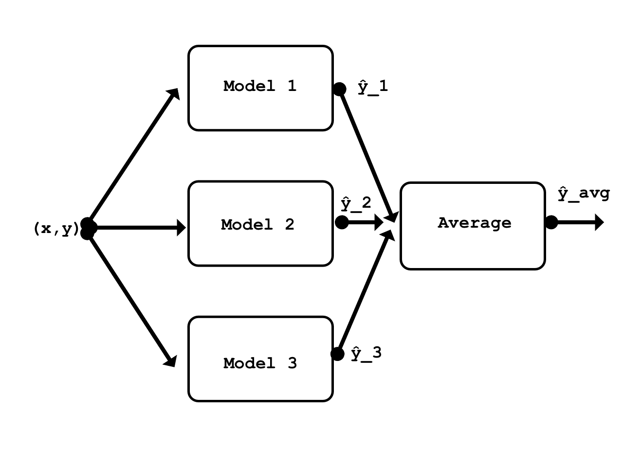
Ensemble diagram
Preparing the data
First, import dependencies.
from keras.models import Model, Input
from keras.layers import Conv2D, MaxPooling2D, GlobalAveragePooling2D, Dropout, Activation, Average
from keras.utils import to_categorical
from keras.losses import categorical_crossentropy
from keras.callbacks import ModelCheckpoint, TensorBoard
from keras.optimizers import Adam
from keras.datasets import cifar10

import numpy as np
I am using CIFAR-10, since it is relatively easy to find papers describing architectures that work well on this dataset. Using a popular dataset also makes this example easily reproducible.
Here the dataset is imported. Both train and test image data is normalized. The training label vector is converted to a one-hot-matrix. Don’t need to convert the test label vector, since it won’t be used during training.
(x_train, y_train), (x_test, y_test) = cifar10.load_data()
x_train = x_train / 255.
x_test = x_test / 255.
y_train = to_categorical(y_train, num_classes=10)
The dataset consists of 60000 32x32 RGB images from 10 classes. 50000 images are used for training/validation and the other 10000 for testing.
print('x_train shape: {} | y_train shape: {}\nx_test shape : {} | y_test shape : {}'.format(x_train.shape, y_train.shape,
                                                                                          x_test.shape, y_test.shape))
x_train shape: (50000, 32, 32, 3) | y_train shape: (50000, 10)
x_test shape : (10000, 32, 32, 3) | y_test shape : (10000, 1)
Since all three models work with the data of the same shape, it makes sense to define a single input layer that will be used by every model.
input_shape = x_train[0,:,:,:].shape
model_input = Input(shape=input_shape)
First model: ConvPool-CNN-C
The first model that I am going to train is ConvPool-CNN-C [4]. Its descritption appears on page 4 of the linked paper.
The model is pretty straightforward. It features a common pattern where several convolutional layers are followed by a pooling layer. The only thing about this model that might be unfamiliar to some people is its final layers. Instead of using several fully-connected layers, a global average pooling layer is used.
Here is a brief overview of how global pooling layer works. The last convolutional layer Conv2D(10, (1, 1)) outputs 10 feature maps corresponding to ten output classes. Then the GlobalAveragePooling2D() layer computes spatial average of these 10 feature maps, which means that its output is just a vector with a lenght 10. After that, a softmax activation is applied to that vector. As you can see, this method is in some way analogous to using FC layers at the top of the model. You can read more about global pooling layers and their advantages in 5 paper.
One important thing to note: there’s no activation function applied to the output of the final Conv2D(10, (1, 1)) layer, since the output of this layer has to go through GlobalAveragePooling2D() first.
def conv_pool_cnn(model_input):

    x = Conv2D(96, kernel_size=(3, 3), activation='relu', padding = 'same')(model_input)
    x = Conv2D(96, (3, 3), activation='relu', padding = 'same')(x)
    x = Conv2D(96, (3, 3), activation='relu', padding = 'same')(x)
    x = MaxPooling2D(pool_size=(3, 3), strides = 2)(x)
    x = Conv2D(192, (3, 3), activation='relu', padding = 'same')(x)
    x = Conv2D(192, (3, 3), activation='relu', padding = 'same')(x)
    x = Conv2D(192, (3, 3), activation='relu', padding = 'same')(x)
    x = MaxPooling2D(pool_size=(3, 3), strides = 2)(x)
    x = Conv2D(192, (3, 3), activation='relu', padding = 'same')(x)
    x = Conv2D(192, (1, 1), activation='relu')(x)
    x = Conv2D(10, (1, 1))(x)
    x = GlobalAveragePooling2D()(x)
    x = Activation(activation='softmax')(x)

    model = Model(model_input, x, name='conv_pool_cnn')

    return model
conv_pool_cnn_model = conv_pool_cnn(model_input)
For simplicity’s sake, each model is compiled and trained using the same parameters. Using 20 epochs with a batch size of 32 (1250 steps per epoch) seems sufficient for any of the three models to get to some local minima. Randomly chosen 20% of the training dataset is used for validation.
def compile_and_train(model, num_epochs):

    model.compile(loss=categorical_crossentropy, optimizer=Adam(), metrics=['acc'])
    filepath = 'weights/' + model.name + '.{epoch:02d}-{loss:.2f}.hdf5'
    checkpoint = ModelCheckpoint(filepath, monitor='loss', verbose=0, save_weights_only=True,
                                                 save_best_only=True, mode='auto', period=1)
    tensor_board = TensorBoard(log_dir='logs/', histogram_freq=0, batch_size=32)
    history = model.fit(x=x_train, y=y_train, batch_size=32,
                     epochs=num_epochs, verbose=1, callbacks=[checkpoint, tensor_board], validation_split=0.2)
    return history
It takes about 1 min to train this and the next model for one epoch using a single Tesla K80 GPU. Training might take a while if you are using a CPU.
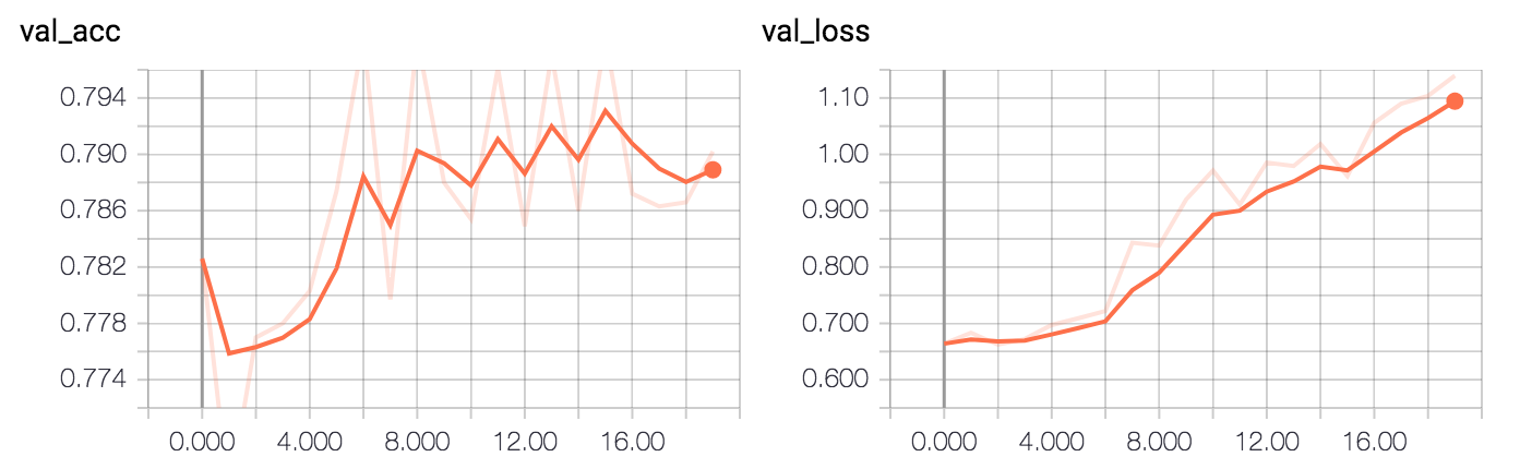
_ = compile_and_train(conv_pool_cnn_model, num_epochs=20)
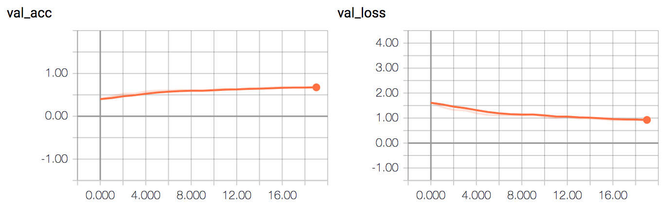
The model achieves ~79% validation accuracy (the plots show validation accuracy/loss vs epoch #).
One simple way to evaluate the model is to calculate the error rate on the test set.
def evaluate_error(model):
    pred = model.predict(x_test, batch_size = 32)
    pred = np.argmax(pred, axis=1)
    pred = np.expand_dims(pred, axis=1) # make same shape as y_test
    error = np.sum(np.not_equal(pred, y_test)) / y_test.shape[0]
    return error
evaluate_error(conv_pool_cnn_model)
0.2414
Second model: ALL-CNN-C
The next CNN, ALL-CNN-C, comes from the same paper [4]. This model is very similar to the previous one. Really, the only difference is that convolutional layers with a stride of 2 are used in place of max pooling layers. Again, note that there is no activation function used immediately after the Conv2D(10, (1, 1)) layer. The model will fail to train if a relu activation is used immediately after that layer.
def all_cnn(model_input):

    x = Conv2D(96, kernel_size=(3, 3), activation='relu', padding = 'same')(model_input)
    x = Conv2D(96, (3, 3), activation='relu', padding = 'same')(x)
    x = Conv2D(96, (3, 3), activation='relu', padding = 'same', strides = 2)(x)
    x = Conv2D(192, (3, 3), activation='relu', padding = 'same')(x)
    x = Conv2D(192, (3, 3), activation='relu', padding = 'same')(x)
    x = Conv2D(192, (3, 3), activation='relu', padding = 'same', strides = 2)(x)
    x = Conv2D(192, (3, 3), activation='relu', padding = 'same')(x)
    x = Conv2D(192, (1, 1), activation='relu')(x)
    x = Conv2D(10, (1, 1))(x)
    x = GlobalAveragePooling2D()(x)
    x = Activation(activation='softmax')(x)

    model = Model(model_input, x, name='all_cnn')

    return model
all_cnn_model = all_cnn(model_input)
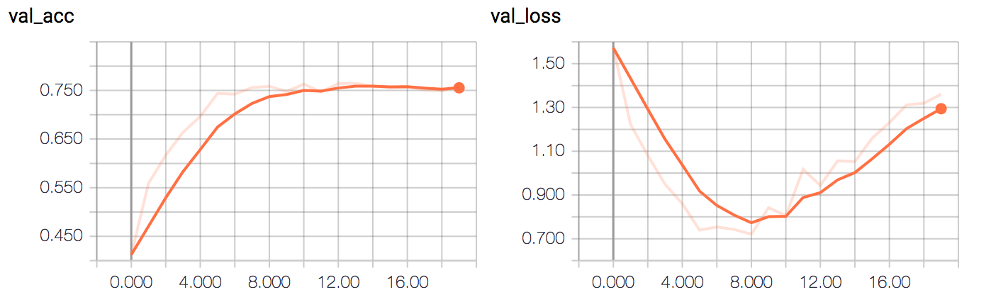
_ = compile_and_train(all_cnn_model, num_epochs=20)
The model converges to ~75% validation accuracy.
Since two models are very similar to each other, it is expected that the error rate doesn’t differ much.
evaluate_error(all_cnn_model)
0.26090000000000002
Third Model: Network In Network CNN
The third CNN is Network in Network CNN [5]. This is a CNN from the paper that introduced global pooling layers. It’s smaller than previous two models, therefore is much faster to train. No relu after the final convolutional layer!
def nin_cnn(model_input):

    #mlpconv block 1
    x = Conv2D(32, (5, 5), activation='relu',padding='valid')(model_input)
    x = Conv2D(32, (1, 1), activation='relu')(x)
    x = Conv2D(32, (1, 1), activation='relu')(x)
    x = MaxPooling2D((2,2))(x)
    x = Dropout(0.5)(x)

    #mlpconv block2
    x = Conv2D(64, (3, 3), activation='relu',padding='valid')(x)
    x = Conv2D(64, (1, 1), activation='relu')(x)
    x = Conv2D(64, (1, 1), activation='relu')(x)
    x = MaxPooling2D((2,2))(x)
    x = Dropout(0.5)(x)

    #mlpconv block3
    x = Conv2D(128, (3, 3), activation='relu',padding='valid')(x)
    x = Conv2D(32, (1, 1), activation='relu')(x)
    x = Conv2D(10, (1, 1))(x)

    x = GlobalAveragePooling2D()(x)
    x = Activation(activation='softmax')(x)

    model = Model(model_input, x, name='nin_cnn')

    return model
nin_cnn_model = nin_cnn(model_input)
This model trains much faster - 15 seconds per epoch on my machine.
_ = compile_and_train(nin_cnn_model, num_epochs=20)
The model achieves ~65% validation accuracy.
This is more simple than the other two, so the error rate is a bit higher.
evaluate_error(nin_cnn_model)
0.31640000000000001
Three Model Ensemble
Now all three models will be combined in an ensemble.
Here, all three models are reinstantiated and the best saved weights are loaded.
conv_pool_cnn_model = conv_pool_cnn(model_input)
all_cnn_model = all_cnn(model_input)
nin_cnn_model = nin_cnn(model_input)

conv_pool_cnn_model.load_weights('weights/conv_pool_cnn.29-0.10.hdf5')
all_cnn_model.load_weights('weights/all_cnn.30-0.08.hdf5')
nin_cnn_model.load_weights('weights/nin_cnn.30-0.93.hdf5')

models = [conv_pool_cnn_model, all_cnn_model, nin_cnn_model]
Ensemble model definition is very straightforward. It uses the same input layer thas is shared between all previous models. In the top layer, the ensemble computes the average of three models’ outputs by using Average() merge layer.
def ensemble(models, model_input):

    outputs = [model.outputs[0] for model in models]
    y = Average()(outputs)

    model = Model(model_input, y, name='ensemble')

    return model
ensemble_model = ensemble(models, model_input)
As expected, the ensemble has a lower error rate than any single model.
evaluate_error(ensemble_model)
0.2049
Other Possible Ensembles
Just for completeness, we can check performance of ensembles that consist of 2 model combinations.
pair_A = [conv_pool_cnn_model, all_cnn_model]
pair_B = [conv_pool_cnn_model, nin_cnn_model]
pair_C = [all_cnn_model, nin_cnn_model]
pair_A_ensemble_model = ensemble(pair_A, model_input)
evaluate_error(pair_A_ensemble_model)
0.21199999999999999
pair_B_ensemble_model = ensemble(pair_B, model_input)
evaluate_error(pair_B_ensemble_model)
0.22819999999999999
pair_C_ensemble_model = ensemble(pair_C, model_input)
evaluate_error(pair_C_ensemble_model)
0.2447
Conclusion
To reiterate what was said in the introduction: every model has its own weaknesses. The reasoning behind using an ensemble is that by stacking different models representing different hypotheses about the data, we can find a better hypothesis that is not in the hypothesis space of the models from which the ensemble is built.
By using a very basic ensemble, a much lower error rate was achieved than when a single model was used. This proves effectiveness of ensembling.
Of course, there are some practical considerations to keep in mind when using an ensemble for your machine learning task. Since ensembling means stacking multiple models together, it also means that the input data needs to be forward-propagated for each model. This increases the amount of compute that needs to be performed and, consequently, evaluation (predicition) time. Increased evaluation time is not critical if you use an ensemble in research or in a Kaggle competition. However, it is a very critical factor when designing a commercial product. Another consideration is increased size of the final model which, again, might be a limiting factor for ensemble use in a commercial product.
You can get the Jupyter notebook source code from my GitHub.
References
- Ensemble Learning. (n.d.). In Wikipedia. Retrieved December 12, 2017, from https://en.wikipedia.org/wiki/Ensemble_learning
- D. Opitz and R. Maclin (1999) “Popular Ensemble Methods: An Empirical Study”, Volume 11, pages 169–198 (available at http://jair.org/papers/paper614.html)
- Learning Multiple Layers of Features from Tiny Images, Alex Krizhevsky, 2009.
- arXiv:1412.6806v3 [cs.LG]
- arXiv:1312.4400v3 [cs.NE]